Image Processing and Analysis in R
Performing Image processing and analysis in R, installation of EBImage package is required. Execute the below code to get package installed in R.
source("http://bioconductor.org/biocLite.R")
 biocLite()
 biocLite("EBImage")
Performing the Reading, Writing and displaying of Image
The loading of package will be done by using the below command.
library (EBImage)Reading Image:The readImage function is used to read Image from file location or URLs
Image <- readImage("C:\\Users\\Public\\Pictures\\Sample Pictures\\ Penguins.jpg")
Displaying Image: Image can be displayed using display function and pixel intensities should range from 0 (black) to 1 (white)
display (Image)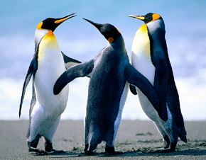
Writing Image: WriteImage function is used to write the Image at a particular location.
writeImage(Image, 'E:\\imgc.jpeg' ,quality=85)Image Properties
Images are stored as multi-dimensional arrays containing the pixel intensities, so if we use the print function it will return the image properties. In the below output two section is present i.e. summary and array of pixels.
>print(Image)
Image
  colorMode    : Color
  storage.mode : double
  dim          : 1024 768 3
  frames.total : 3
  frames.render: 1

imageData(object)[1:5,1:6,1]
          [,1]      [,2]      [,3]      [,4]      [,5]      [,6]
[1,] 0.4549020 0.4549020 0.4627451 0.4588235 0.4666667 0.4745098
[2,] 0.4627451 0.4549020 0.4588235 0.4588235 0.4627451 0.4666667
[3,] 0.4627451 0.4588235 0.4588235 0.4627451 0.4588235 0.4588235
[4,] 0.4705882 0.4627451 0.4627451 0.4627451 0.4627451 0.4627451
[5,] 0.4627451 0.4549020 0.4627451 0.4627451 0.4627451 0.4666667
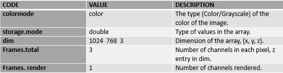
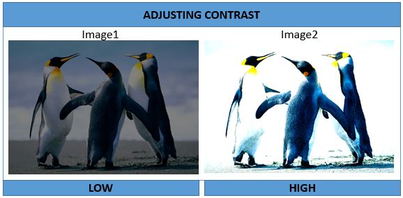
Image matrices operation for Adjusting Brightness, Contrast and Gamma correction
Image matrices obtained values from mapping pixels in the image to the real line between 0 and 1. Both extremes of this interval [0, 1], are black and white colours, respectively. Hence, pixels with values closer to any of these end points are expected to be darker or lighter, respectively. And because pixels are contained in a large array, then we can do all matrix manipulations available in R for processing.
As matrices, images can be manipulated with all R mathematical operators. For image sitting control can be achieved using mathematical operators.
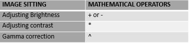
Adjusting Brightness
Image1 <- Image + 0.2
Image2 <- Image - 0.2
display (Image1); display(Image2)
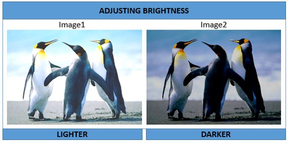
Image1 <- Image * 0.5
Image2 <- Image * 2
display(Image1); display(Image2)
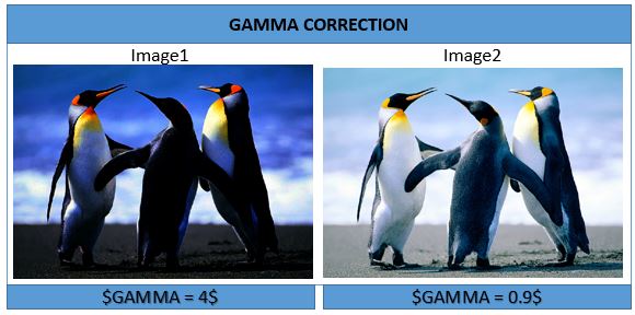
Gamma Correction
Image1 <- Image ^ 4
Image2 <- Image ^ 0.9
display(Image1); display(Image2)
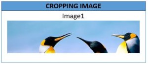
Cropping Image
Image1 <-Image[1:800, 1:200,]
display(Image1)
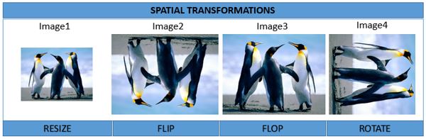
Spatial Transformation
Spatial image transformations can be performed with the functions such as re-size, rotate, translate and the functions flip and flop to reflect images.
#Resizing the image
Image1 <- resize(Image, 500)
display(Image1)
# FLip and Flop of image
Image2 <- flip(Image)
display(Image2)
Image3 = flop(Image)
display(Image3)
#Image Rotation
Image4 <- translate(rotate(Image, 90), c(50, 0))
display(Image4)
The function colorMode can access and change the value of the slot colormode, altering the rendering mode of an image. In this, the Color image (Image) with one frame is changed into a Grayscale, corresponding to the red, green and blue channels.
>print(Image)
Image
  colorMode    : Color
  storage.mode : double
  dim          : 1024 768 3
  frames.total : 3
  frames.render: 1

imageData(object)[1:5,1:6,1]
          [,1]      [,2]      [,3]      [,4]      [,5]      [,6]
[1,] 0.4549020 0.4549020 0.4627451 0.4588235 0.4666667 0.4745098
[2,] 0.4627451 0.4549020 0.4588235 0.4588235 0.4627451 0.4666667
[3,] 0.4627451 0.4588235 0.4588235 0.4627451 0.4588235 0.4588235
[4,] 0.4705882 0.4627451 0.4627451 0.4627451 0.4627451 0.4627451
[5,] 0.4627451 0.4549020 0.4627451 0.4627451 0.4627451 0.4666667

>#Greyscale Image
>colorMode(Image) <- Grayscale
>display(Image)
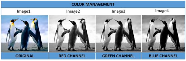
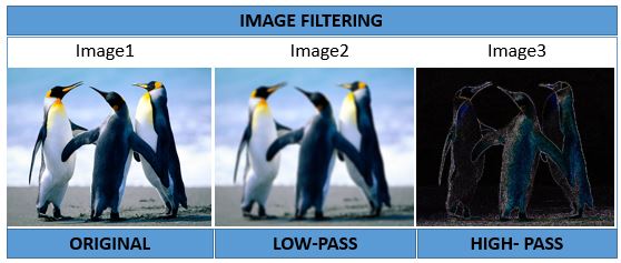
Image Filtering
Images can be linearly filtered using filter2. Low-pass filtering is used to perform blur image, remove noise, etc. High-pass filtering is used to perform detect edges, sharpen images etc., various filter shapes can be generated using makeBrush.
#LOW-PASS Filtering image
flo = makeBrush(21, shape='disc', step=FALSE)^2
flo = flo/sum(flo)
imgflo = filter2(Image, flo)
display(imgflo)
#HIGH-PASS Filtering image
fhi = matrix(1, nc=3, nr=3)
fhi[2,2] = -8
imgfhi = filter2(Image, fhi)
display(imgfhi)
Equalize the image histogram to a specified range and number of levels. Individual channels of Color images and frames of image stacks are equalized separately.
y= equalize(Image) hist(y)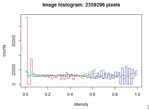
References
1) http://www.bioconductor.org/packages/release/bioc/manuals/EBImage/man/EBImage.pdf
2) http://www.r-bloggers.com/r-image-analysis-using-ebimage/
3) http://www.bioconductor.org/packages/release/bioc/vignettes/EBImage/inst/doc/EBImage-introduction.pdf
Write a comment
- M12MOUNT LENSES July 27, 2015, 12:10 pmI like your blog.I enjoyed reading your blog.It was amazing.Thanks a lot. http://www.balaji-microtechnologies.com/balaji-optics-megapixel-board-camera-lenses.htmlreply
Subscribe To Our Newsletter
Join our mailing list to receive the latest blogs and updates.